Why Good Forecasts Treat Human Input as Part of the Model

At DoorDash, getting forecasting right is critical to the success of our logistics-driven business, but historical data alone isn’t enough to predict future demand. We need to ensure there are enough Dashers, our name for delivery drivers, in each market for timely order delivery. And even though it seems like people’s demand for food delivery should be just as regular as the number of meals they eat in a day, there is a lot of variation in how often consumers decide to order from DoorDash, which makes it difficult to get an accurate forecast. 

Because of the variance of the historical data we use to train our models, we often need to add different types of  human input to our forecasts to make them more accurate. For example, input from our marketing team is helpful because DoorDash is constantly trying out new marketing strategies, and these team members already know what impact to expect. Every time there is a holiday, a major promotion, or even some rain, the behavior of our consumers can shift dramatically in unexpected ways. While our models take most such events into account, any big, trend-breaking event can have a significant negative impact on the future accuracy of our forecasting model and be detrimental to the overall user experience. 

The rarity of these events also makes it impractical to encode them into our models. In many cases, forecasting accurately can be as much about the ability to engineer an incredible machine learning (ML) model as it is about asking our marketing teams what they think is going to happen next week and figuring out how to incorporate that assessment into our forecast.

In general, we’ve found that the best approach is to separate our forecasting workflow into small modules. These modules fall into one of two categories, preprocessing the data or making an adjustment on top of our initial prediction. Each module is narrow in scope and targets a specific contributor to variance in our forecast, like weather or holidays. This modular approach also comes with the advantage of creating components that are easier to digest and understand.

Once we’ve done the groundwork to build a model that correctly estimates the trajectory of our business, our stakeholders and business partners add an extra level of accuracy. Building pipelines that support the rapid ingestion and application of business partner inputs plays a big part in making sure that input is effective. This line of development is frequently overlooked and should generally be considered part of the forecasting model itself.

Preprocessing the data

Preprocessing involves smoothing out and removing all the irregularities from the data so that the ML model can infer the right patterns. For example, let’s say we have a sustained marketing campaign which results in weekly order numbers growing 10% for the next few weeks. If we were expecting seasonal growth to be 5% then we should attribute this extra growth to the marketing campaign and adjust future weeks’ demand to be lower as the marketing campaign loses steam.

Smoothing can be done by using algorithms to automatically detect and transform outliers into more normal values or by manually replacing the bumps in our training data with values derived with some simple method. Using an algorithm to smooth out the data can work really well, but it is not the only way to preprocess the data. There are often some elements of the series that cannot be smoothed well that need to be handled with manual adjustments. These can include one-time spikes due to abnormal weather conditions, one-off promotions, or a sustained marketing campaign that is indistinguishable from organic growth.

How replacing outliers manually in training data can lead to better accuracy

At DoorDash we’ve learned that holidays and other events highly influence the eating habits of our consumers. Making sure that we’re building a forecast off of the correct underlying trends is critical to creating an accurate demand forecast. An important part of building a predictive model is creating a training set that reduces the variance and noise of everyday life,  thereby making it easier for the model to detect trends in the data. Figure 1, below, shows a typical time series (a sequence of data points ordered by time) at DoorDash.

Our data looks somewhat sinusoidal, a wave-like shape defined by periodic intervals that alternate between a peak and a trough, with the peaks and the troughs of the wave series being somewhat irregular. There is a huge dip in the middle of the series that doesn’t match the pattern at all. That dip is typical of a holiday where demand dips, but is an outlier compared to normal ordering behavior.

Here are a few different preprocessing methods we might use before training our model: 

• Training the model as-is with no pre-processing:
  • We will be training the model on the raw data using the ETS algorithm, which has the exponential smoothing algorithm built into the forecast.
  • These results will be our baseline so we can see how additional preprocessing adds accuracy.
• Use another smoothing algorithm on top of what’s built into the ETS model: 
  • In this instance we are using the Kalman filter from tsmoothie, an algorithm from the package that helps smooth time series data. We chose this algorithm specifically because it takes in parameters that help adjust for seasonality and trends.
• Make some manual adjustments to the training set:  
  • This method uses human intuition to recognize that for every dip, there was a broad change to consumer behavior. These changes are caused by a combination of holidays and promotions that are not random variance. For the current example, the best solution is to replace the outlier week with the most recent week prior to the dip as a proxy for what should have happened.
• Use both manual adjustments and a smoothing algorithm:
  • This final method uses the manual adjustment approach and smooths the result afterwards.

All three of the methods made noticeable changes compared to the shape of the raw data, as shown in Figure 2, above. The Kalman filter couldn’t quite approximate the sinusoidal shape in the extreme dip but it did smooth the curve out a bit. The manual adjustments did a great job of approximating the shape as well, but didn’t flatten out that spike on day 32. The manual adjustments combined with the Kalman filter exhibit slightly different behavior in peaks and troughs and exhibit a more normal sine wave pattern overall.

The results

After preprocessing the training data and then training a model, we can see that each method yielded a noticeably different prediction.

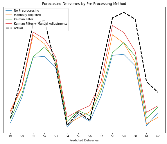
Method	Error Reduction Relative to No Preprocessing (Higher is Better)
Manually Adjusted	19%
Kalman Filter	15%
Kalman Filter + Manually Adjusted	35%

We see that both the Kalman filter and the manually adjusted method yielded improvements over the untreated data. But in this case the combination of the manual adjustments and the Kalman filter ended up yielding an even better result than either method individually. This example shows that by employing a couple of simple pre-processing methods, we can get increased accuracy in our models.

Adjusting the predictions of the forecast to improve accuracy 

Making adjustments to our predictions involves the integration of smaller individual modules that take into account a variety of factors that swing DoorDash’s order volume, with some of the biggest factors being weather and holidays. While we can try and create models that address things like weather or holidays, there will always be trend-breaking events that can’t be modeled. Turning to human input can improve the model’s accuracy at this stage.

Why not just build a better model with more inputs?

Building a bigger and better model ends up not being practical because it’s not really possible to account for every use case. For example, in September of 2019  we gave away one million Big Macs. DoorDash at that point had been giving promotions to customers regularly, but never on that scale. There wasn’t a good way to handle this new scenario with a model that predicts the effect of promotions since the scale and scope were just completely different from our usual promotions, which are what we would have used for training data.

We initially chalked this up as a one-time event, thinking that it wasn’t necessary to design for such an infrequent promotion, but events of this nature kept happening. Just a few months later, we partnered with Chase to offer DashPasses to many of their credit card holders, and got a massive influx of traffic as a result. 

In the face of a major event like this, we could only make one of three choices:

• Expect that the impact of large promotional events is not so large that we cannot deliver all our orders. 
• Build a generic promotional model and hope the results generalize to future outliers. 
• Get input from the team running the relevant promotions to boost our accuracy with manual intervention.

Option one is extremely unlikely, and is not in the spirit of trying to improve a model’s accuracy, since it's to the detriment of our marketing team’s performance. Option two would give marginal results at best, and given that every major promotion can be different, finding a feature set that can generalize well to outlier events like these is unlikely. Option three often ends up being the only choice, because the business teams that set up these promotions have spent a lot of time sizing up their impact and already have a good estimate on the impact.

In practice, we begin option three by building out the infrastructure that enables a forecast to ingest adjustments that manually alter the forecast. Although the adjustments can end up being something simple, like adding an extra 100,000 deliveries to Saturday’s forecast, there can still be cascading problems to solve. For example, if we adopted the simple example above there would need to be methods or models in place to figure out how to distribute that extra 100,000 deliveries to all our geographies. But once the code is in place to rapidly propagate manual adjustments, each manual adjustment should just feel like adding another input to the model. In this way we can ask business teams their opinions on upcoming forecasts and easily incorporate those into our forecasting model.  

Conclusion

Like most machine learning problems, forecasting requires a real understanding of a problem’s context before throwing computing power and algorithms at it. A simple solution, like getting input from business partners, can end up improving forecasting accuracy just as much as using a complex algorithmic solution. That is why enabling the input of  experts or stakeholders at the company can help improve the forecast’s accuracy even more.