Maintaining Machine Learning Model Accuracy Through Monitoring

Machine learning (ML) models give us reliable estimates for the time it takes a restaurant to prepare a food order or how long it will take an order to reach a consumer, among other important metrics. However, once an ML model is trained, validated, and deployed to production, it immediately begins degrading, a process called model drift. This degradation negatively impacts the accuracy of our time estimates and other ML model outputs.

Because ML models are derived from data patterns, their inputs and outputs need to be closely monitored in order to diagnose and prevent model drift. Systematically measuring performance against real-world data lets us gauge the extent of model drift.

Maintaining an optimal experience for our platform users required developing observability best practices to our ML models at a system level to detect when a model was not performing as it should. We approached model observability as an out-of-the-box monitoring solution that we can apply to all of our ML models to protect the integrity of their decision making.

Why we invested in model observability 

The typical ML development flow involves feature extraction, model training, and model deployment. However, model monitoring, one of the most important steps, only starts after a model is deployed. Monitoring a model is important because model predictions often directly influence business decisions, such as which deliveries we offer to Dashers (our term for delivery drivers).

Model predictions tend to deviate from the expected distribution over time. This deviation occurs because, with more customers, more products, and more orders on our platform, the data patterns change. For example, a shift could be the result of an external event, such as the COVID-19 pandemic, which caused a huge shift in how customers interacted with DoorDash. 

In the past, we’ve seen instances where our models became out-of-date and began making incorrect predictions. These problems impacted the business and customer experience negatively and forced the engineering team to spend a lot of effort investigating and fixing them. Finding this kind of model drift took a long time because we did not have a way to monitor for it .

This experience inspired us to build a solution on top of our ML platform. We set out to solve this model drift problem more generally and avoid issues like it in the future for all of the ML use cases on our platform. Ultimately, our goal was to create a solution that would protect all the different ML models DoorDash had in production. 

An overview of our ML platform

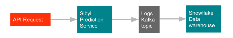
Within DoorDash’s ML platform, we have Sibyl, a prediction service, that logs all predictions, as described in Figure 1, below:

Whenever our data scientists wanted to investigate the performance of a model, the prediction logs would be useful. The prediction logs consist of every prediction made by a model, including the prediction result, prediction ID, feature values, and object identifiers that were used to make that prediction. Combining the prediction logs and the model artifact, a data scientist should be able to fully reproduce the model’s prediction.

We store these prediction logs in a data warehouse easily accessible to our data scientists. While this storage methodology made deep dives easy, it did not help in understanding the big picture of why models were drifting. We needed a more specific ML model monitoring solution.

Choosing an ML model monitoring approach

When we approached the problem of how to monitor our ML models, we took a systems thinking approach to MLOps (an approach to operationalizing machine learning). We considered features (ML model inputs) and predictions (ML model outputs) as two key components. To begin designing our solution, we surveyed existing open source approaches and interviewed our data scientists on what kind of information they would like to see for model monitoring. The information we gathered made it clear that statistical monitoring can be applied to both features and predictions.

When we surveyed existing open source projects and industry best practices, two distinct approaches emerged: a unit test approach and a monitoring approach. The difference between the two approaches can be explained in terms of writing software. We can write unit tests to test the functionality and robustness of software, and we can implement monitoring systems to observe production performance. These approaches are complementary, and the question of data monitoring and model monitoring in the open source arena ends up with a solution in either one of these buckets.

Approach	Expectations	Adoption	Parity between training and production
Unit test	Pass/fail status	Opt-in	Assumes training data will match production data
Monitoring	Trends distribution	Out-of-the-box	Does not assume that training data will match production data

In the unit test approach, the data scientist opts in by analyzing the data, deciding the validations (such as, “I expect delivery time to be not more than one hour”), and recording these validations. These validations are then run on all new data. In the preceding example, the validation checks every delivery time input to be under one hour. However the introduction of new products can change this assumption, so the data scientist will be alerted that inputs have changed.

In the monitoring approach, we use DevOps best practices, generating metrics via standard DevOps tools such as Prometheus and monitoring using charts via tools such as Grafana. Prometheus’ Alertmanager can be set to send alerts when metrics exceed a certain threshold.

Let’s compare the two approaches based on their setting of expectations, requirements of adoption, and assumption of parity between training and production data.

Setting expectations 

In terms of setting expectations, the upside of the unit test approach is that these validations will crystallize the data scientists’ expectations of the expected inputs and outputs of their models. The downside is that these validations are Boolean, meaning they either pass or fail, which does not help the data scientist diagnose the underlying issue. 

For example, this unit test approach will not provide details if data transitions from a gradual to a sudden change.  It will only send an alert when certain metrics are exceeded. The reverse is true for the monitoring approach. There are no preset expectations to judge against, but the trends in the data are visible during analysis.

Requirements of adoption 

In terms of adoption, the upside of the unit test approach is that data scientists have flexibility in choosing the validations on the inputs and outputs of the model. The downside is that  unit tests are opt-in, requiring explicit effort from data scientists to adopt them. In the monitoring approach, the system can generate these metrics automatically but there is less flexibility in what validations are chosen.

Assumption of parity between training and production 

In terms of parity between training and. production, the unit test approach expects training data to match production values. The downside of this assumption is that, in our internal survey, data scientists do not assume parity between training and production data. They expect production data to be different from training data from the first day that a model is deployed to production. 

Allowing for a difference in training and production data means that the unit test approach could generate alerts on launch day. These alerts may be false because perfect parity between training data and production data is difficult in practice. In the monitoring approach, there are no preset expectations and data is immediately available for analysis as well as on an ongoing basis.

Choosing the best approach 

Given these tradeoffs, we decided to ask the team for their preferences between these two approaches. We prepared a questionnaire and interviewed our data scientists on what functionalities they are looking for, and asked them to stack and rank their must-haves with their nice-to-haves. After collecting the survey responses  it became clear that they wanted to see trends distribution, would prefer a platform solution, and did not assume that training data will match production data.

Given the use cases by data scientists, we decided to adopt the monitoring approach. To implement monitoring, we needed three steps: generate the relevant metrics, create a dashboard with graphs, enable alerting on top of these metrics. 

The monitoring approach gave us the following benefits:

1. Leveraging existing tools: We can design a configurable, scalable, flexible platform for displaying metrics and setting up alerts by reusing tools provided by the Observability team.
2. No onboarding required: Data scientists don’t need to individually write code to add monitoring to their training pipeline and do not have to think about the scalability and reliability of the monitoring solution. 
3. Open source standards: By using standard open source observability tools such as Prometheus and Grafana, data scientists and engineers do not need to learn a homegrown system.
4. Easy visualization: Graphing tools such as Grafana offer the ability to interactively view splits and historical data. This is an incredibly useful tool when it comes to finding correlations between events.
5. Self-service: Data scientists can use this tool without the help of the platform team, which ensures a more scalable detection of model drift going forward.

Building ML model monitoring as a DevOps system

After choosing the monitoring approach, we had to decide what technology stack to use in order to leverage DoorDash’s existing systems. As shown in Figure 1, above, we could monitor the data at the Apache Kafka topic step or at the final data warehouse step. We decided to use the data warehouse step for the first release because we could leverage SQL queries. We could build our second release on top of our real-time processing system, giving us the benefit of real-time monitoring.

Our prediction logs are continuously uploaded to our data warehouse. The schema of the data is:

• sent_at : timestamp
  • The time when the prediction was made.
  • We use this timestamp for aggregations in our monitoring. It’s also important to distinguish between multiple predictions made on the same features by the same model.
• prediction_id : string
  • User-supplied identifier for which object the prediction was made on. This can be a matching delivery ID, user ID, merchant ID, etc.
• predictor_name : string
  • A predictor name is the purpose, e.g. ETA prediction.
  • A predictor name can be configured to map to a default model ID as well as shadow model IDs.
  • The shadow models will result in additional predictions made and logged.
  • Shadow models are used to monitor behavior and when behavior matches expectations, they can be promoted to a default model ID.
• model_id : string
  • The versioned name of the ML model trained to perform predictions. ML modeling is an iterative process so we need to keep track of model versions over time.
• features : key-value pairs
  • Each feature name is accompanied by its corresponding feature value.
• prediction_result : numerical
  • The output of the ML model that will be used by the caller service.
• default_values_used : set of feature names
  • If an actual feature value was unavailable, we fallback to the default feature value configured in the model, and we note the same by adding the feature name to this set.

As part of our user research, data scientists told us they worried about what percentage of predictions used default values, as it was a leading indicator of low feature coverage. Sibyl, our prediction service, would use default values specified in the model configuration files whenever specific values were unavailable. For example, it would use a default meal preparation time if we do not know the average meal preparation time for a specific restaurant. 

Sibyl inputs default values in real-time while making predictions. However, at the time of monitoring we do not know the default aggregate values. In order to find out how often we used default values, we added functionality in Sibyl to also log whenever a default value was used.

We combined this schema with SQL aggregation functions, such as avg, stddev, min, max, and approx_percentile (e.g. P5, P25, P50, P75, P95), to create SQL query templates.

Monitoring tasks can be created using YAML configuration files that define the monitoring cadence, and the types of metrics we want to extract from each model and predictor.

Both hourly and daily we plug in the duration, the predictor name, and the model ID into this SQL query template, generate the final SQL, query the data warehouse, and, once we receive the aggregated value, emit this information as a Prometheus metric.

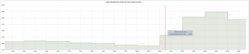
Once the Prometheus metrics are available, our data scientists and machine learning engineers can make full use of the platform. For example, we can view the trends of feature value statistics using the Grafana dashboard, which includes graphs for a specific predictor name, model ID and feature name, as shown in Figure 2, below:

We were able to leverage our internal Terraform repository for alerting, where we can create queries using PromQL, add thresholds, and connect alerts to either a team-specific Slack channel or a team-specific PagerDuty. Our Observability team already used this infrastructure, making the path of model monitoring smooth and easy to adopt, since it was not a new tool for our data scientists and engineers to learn.

Improvements of flexibility and coverage

With this first release, we had a fully functional monitoring, graphing, and alerting workflow for detecting model drift. Thanks to close consulting and coordination with data scientists, we were able to onboard many teams, including our Logistics, Fraud, Supply and Demand, and ETA teams, for the first release.

Based on their usage and feedback, we made several improvements.

In our first release, we enabled monitoring flexibility for data scientists by allowing them to configure the specific metrics they wanted for specific feature names. This addition had the drawback of requiring an onboarding step for new models and new feature names. In our second release, we enabled complete monitoring for all models, all feature names, and all metrics, thereby eliminating the onboarding step. This second release achieved our vision of an out-of-the-box experience.

In our first release, we calculated statistics at both the hourly and daily aggregation level. It turns out that hourly is far more valuable than daily, since we see peaks around lunch and dinner times, hence there is more value in the distribution than averages. In our second release, we focused exclusively on hourly aggregation, rebuilding the monitoring using our real-time processing pipeline for real-time graphs and alerting.

Another improvement to the output monitoring came with the introduction of opt-in evaluation metrics. While understanding descriptive statistical properties of our predictions is valuable, a more useful metric would tell us how close our predicted values are to the actual values. Is our ML model actually doing a good job of modeling complex problems in real-world applications? For example, when we predict the ETA of a delivery, we can infer the actual delivery time by the difference between when the delivery was placed and when it was delivered.

ML tasks can be categorized based on what type of prediction they make. Each of these tasks require a specialized set of evaluation metrics:

• Regression (mean squared error, root mean square error)
• Classification (accuracy, precision, area under curve)
• Ranking (mean reciprocal rank, normalized discounted cumulative gain)
• Text processing (BLEU score)

There are a few challenges with determining which evaluation metrics to use or how to refine them for our monitoring system. In some applications, such as prep time modeling, the data is censored. In other applications, such as predicting fraudulent orders, the true value might not become available for weeks because the payment processors and banks need to investigate the orders.

One commonality between these two cases is that the predicted and actual values need to be stored separately. Actual values are often available either explicitly or implicitly in our database tables for a given prediction ID. Once we make the connection between the prediction ID and the database row with the actual value, we can build a JOIN query to view them side-by-side and use one of the commonly available evaluation metrics. Some computations can be done using elementary operations, such as mean absolute error, but for more complex metrics, the data can be loaded and evaluated using Apache Spark jobs in a distributed manner.

To summarize, we leveraged the prediction logs emitted by our internal prediction service, created aggregations, emitted descriptive statistics and evaluation metrics as Prometheus metrics, viewed those metrics in Grafana charts, and enabled alerting using our internal Terraform repository for alerts.

Future work

Looking forward, we want to double down on DoorDash’s “1% Better Every Day” value, making incremental improvements to the monitoring system. The exciting work ahead of us includes expanding the scope of the monitoring system to more applications, and improving usability, reliability, and the overall value to data scientists and DoorDash.

Some real-time applications not only benefit from, but also require us to respond to issues more frequently than just on an hourly basis. We will change the data, graphing, and alerting aspects of our system to operate on a continuous time scale.

To extend the power of qualitative metrics, data scientists could compare the training performance of a model to the performance in production. As a best practice, ML practitioners typically set aside an evaluation set during training. Using this same evaluation set, we can verify whether the model is making the predictions as expected. Common mistakes that could cause discrepancies are missing features or incorrect input conversions.

While descriptive statistics and alert thresholds are a powerful tool for catching misconfigurations and sudden changes, a more general approach is necessary for detecting a broader set of regressions. For example, a metric might not experience a sharp change but rather a gradual change over time as a result of changing user behavior and long-term effects. A general area of research that we could tap into is anomaly detection, where we can treat predictions as time-series data and detect outliers that happen over time.

Product engineers and data scientists often iterate on machine learning models and need to understand the product implications of their changes. More often than not, new experiments map one-to-one to new ML models. To streamline the analysis process, we could integrate ML model monitoring with Curie, our experimentation analysis platform.

Oftentimes, ML models can produce unexpected results that can be difficult to interpret, delaying investigations. This is an especially common problem with more complex models such as neural networks. To mitigate this problem, our platform could also expose information about why a certain prediction was made. What were the inputs that contributed most to the outcome? How would the output change if we change a feature value slightly?

Conclusion

We identified a common process in ML model development that we systematized and integrated into our ML platform, thereby achieving our goal of letting data scientists focus on model development rather than systems design.

The DevOps approach to metrics for monitoring model performance has worked well for our customers, DoorDash’s data scientists and machine learning engineers, both in terms of how quickly we were able to deliver something useful as well as the ease-of-use and flexibility. Our customers are able to view the trends in charts, zoom in and out of time ranges, and compare trends across different periods of time. Our customers are also able to create custom self-serve alerting on top of these metrics. We abstracted away the complexity so our customers can focus more on developing ML models that make DoorDash a great experience for customers, merchants, and Dashers.

The model monitoring system is scalable in terms of data size, number of models, number of use cases, and number of data scientists. We leverage our platform to enable monitoring out-of-the-box.

This design and solution has shown benefits for the ML models we use internally that affect our business metrics. We believe this approach is a viable and scalable solution for other data-driven teams who want to prevent issues such as data drift and model drift.

Acknowledgements

The authors would like to thank Kunal Shah, Dhaval Shah, Hien Luu, Param Reddy, Xiaochang Miao, Abhi Ramachandran, Jianzhe Luo, Bob Nugman, Dawn Lu, and Jared Bauman for their contributions and advice throughout this effort.

Header photo by Nate Johnston on Unsplash.