At DoorDash, we want our service to be a daily convenience offering timely deliveries and consistent pricing. Achieving these objectives requires a good balance between the supply of Dashers (our term for delivery drivers) and the demand for orders. 

During periods of high demand we generally increase pay, providing an incentive to ensure enough Dashers are available for consumers to receive their orders as quickly as possible. We do not pass through this increased pay to consumers, who will pay the same fees no matter the time of day. 

Given the complexity of offering Dashers peak demand pay, we built a new mobilization system that allocates incentives ahead of any anticipated supply and demand imbalance. When building this system, we focused on the following things:

• Defining our supply and demand measurement metrics and project objectives clearly
• Generating high-fidelity forecasts for supply and demand
• Setting up a new optimization process for incentive allocation under constraints
• Managing uncertainty 
• Improving reliability and maintainability of the system

How do we quantify supply and demand imbalance?

When outlining the problem of supply and demand imbalance, it is useful to adopt the context of all the affected parties:

• For consumers, a lack of Dasher availability during peak demand is more likely to lead to order lateness, longer delivery times, or inability to request a delivery and having to opt for pick up. 
• For Dashers, a lack of orders leads to lower earnings and longer and more frequent shifts in order to hit personal goals.
• For merchants, an undersupply of Dashers leads to delayed deliveries, which typically results in cold food and a decreased reorder rate.

With this context, it becomes clear that the ideal scenario would be to have a system that balances supply and demand at a delivery level instead of market level, but this is not realistic when choosing market-measurement metrics. Balancing at the delivery level means every order has a Dasher available at the most optimal time and every Dasher hits their pay-per hour target.

In contrast, market-level balance means there are relatively equal numbers of Dashers and orders in a market but there are not necessarily optimal conditions for each of these groups at the delivery level. In practice, the variance level for supply and demand driven by Dasher and consumer preferences and other changing conditions in the environment, such as traffic and weather, make it difficult to balance supply and demand at the delivery level. Hence, we focused on market-level metrics to define the state of each market, even though a delivery-level metric would have provided a more ideal outcome. 

For our primary supply and demand measurement metric, we looked at the number of hours required to make deliveries while keeping delivery durations low and Dasher busyness high. By focusing on hours, we can account for regional variation driven by traffic conditions, batching rates, and food preparation times. 

To understand how this metric would work in practice let's consider an example. Let’s imagine that it is Sunday at dinner time in New York City, and we estimate that 1,000 Dasher hours are needed to fulfill the expected demand. We might also estimate that unless we provide extra incentives, only 800 hours will likely be provided by Dashers organically. Without mobilization actions we would be undersupplied by about 200 hours.

We generally compute this metric where Dashers sign up to Dash and to time units that can span from hourly durations to daypart units like lunch and dinner. It is very important to not select an aggregation level that can lead to artificial demand and supply smoothing. For example, within a day we might be oversupplied at breakfast and undersupplied at dinner. Optimizing for a full day would lead to smoothing any imbalance and generate incorrect mobilization actions.

Once we decide on the health metric and the unit at which we take actions, we proceed with balancing supply and demand through adjustments to supply. Our team generally adjusts the supply side of the market by offering incentives to increase Dasher mobilization when there is more demand. Through incentives, we provide Dashers a guarantee that they will earn a fixed amount of money on any delivery they accept in a specific region-time unit. We will describe in the following section how forecasting and optimization plays a role in that.

How do we forecast supply and demand at a localized level?

Now that we have a metric to measure supply and demand levels, a unit of region/time to take actions, and actions we take to manage supply, we can determine our forecasting requirement details and how we forecast each market’s supply and demand conditions.

Defining forecasting requirements

Given that the forecasts we generate are meant to be used in an automated system, both the algorithm we use for forecasting and the subsequent library ecosystem we would rely on can have a large impact on maintaining automation in the long run. We primarily reformulated the forecasting problem into a regression problem and used gradient boosting through the Microsoft-developed open source LightGBM framework. There are a couple of reasons behind this choice.

Support for multivariate forecasting

Many univariate forecasting approaches do not scale well when it comes to generating thousands of regional forecasts with low-level granularity. Our experience strongly supports the thesis that some of the best models are created through a process of rapid prototyping, so we looked for approaches where going from hypothesizing a model improvement to having the final result can be done quickly. LightGBM can be used to train and generate thousands of regional forecasts within a single training run, allowing us to very quickly iterate on model development. 

Support for extrapolation

As DoorDash expands both nationally and internationally, we need our forecasting system to be able to generate some expectations for how our supply and demand growth would look in places where we don’t currently offer our services. For example, if we launch in a new city, we can still make reasonable projections regarding the supply and demand trajectory even with no historical data. Deep learning and traditional machine learning (ML)-based approaches work particularly well in this case, since latent information that helps with extrapolation can either be learned through embedding vectors or through good feature engineering. Information about population size, general traffic conditions, number of available merchants, climate, and geography can all be used to inform extrapolation.

Support for counterfactuals

Forecasts are used to set an expectation of what will happen but they are also inevitably used to guide the decision-making process. For example, our stakeholders would ask us how conditions would change if we changed incentive levels in our supply forecast model so that we can understand how to make tradeoffs between supply and costs. These types of counterfactuals are very helpful not only in forecasting what we think will happen, but in also estimating the impact of actions we are going to take. In LightGBM, approximate counterfactuals can be generated by changing the inputs that go into the model at inference time. 

Small dependency footprint

We wanted the forecasting system to have a minimal dependency footprint, meaning that we were not overly reliant on a host of third-party libraries. This requirement immediately removed a lot of the auto-forecasting approaches, where installing one library often meant installing 100-plus additional libraries, or approaches that provided unified toolkits and had a large number of transitive dependencies. A bloated footprint creates compatibility issues, upgrade challenges, and a large exposure area to security vulnerabilities. LightGBM has a very small dependency footprint, and it is relatively painless to perform upgrades. 

Thriving community

Lastly, we wanted to rely on an ecosystem with a thriving community and a strong core maintainer group. Maintaining an open source library is challenging. A library might be created by a graduate student or one to three core developers working within a company. Nonetheless, folks find new interests, new jobs, switch jobs, find new careers, or abandon careers. Keeping track of issues and bugs related to a library is often not a priority a few years or months down the line. This eventual lack of support then forces users to create internal forks in order to adopt the forecast tooling for their use cases or engage in a complete remodelling exercise. For these reasons, when selecting a tool, we looked at metrics like release cycles, number of stars, and community involvement to ensure there would be good community maintenance into the future. 

Forecasting with ML

Forecasting in the context of a pure regression problem can have it’s challenges, one of which has to do with understanding the data generation process and the causality between the inputs and outputs. For example, Figure 1, below, shows how our incentives relate to the growth in the number of Dasher hours.

If we blindly rely on the model to learn causality through correlations found in the data, we would’ve created a system that would mistakenly assume that providing very high incentive levels would lead to fewer Dashers on the road. A causal interpretation, where high growth incentives would lead to a decrease in mobilization would be nonsensical. 

It is more likely that the model is simply missing a confounding variable. For example, in periods associated with bad weather or holidays, Dashers want to spend time inside or with their families. We are more likely to see a decrease in availability during these times, triggering our supply and demand systems to offer higher incentives to keep the market balanced. 

A model lacking knowledge of weather or holidays might learn that high incentives lead to fewer Dasher hours, when the causal relationship is simply missing a covariate link. This example illustrates why it becomes important to figure out a way to sometimes constrain relationships found in the data through domain knowledge, or to rely on experimental results to regularize some correlational relationships identified by the model and not blindly apply the algorithm to the available data.  

A second challenge has to do with a common truism found in forecasting, which is that the unit of forecasting needs to match the context at which decisions are made. It can be tempting to forecast even more granularly, but that is generally a bad idea. This can be easily demonstrated through a simulation.

Consider the following three sub-regions describing daily demand by drawing samples, as shown in Figure 2, below, from a normal distribution with a mean of 100 and standard deviation of 25, giving us a coefficient of variation of 25%. When we aggregate these regions, we simply sum the expected mean to get an expected aggregate demand of 300. Nonetheless, the combined standard deviation is not equal with the sum of standard deviations but with the sum of the variances , which gives us a coefficient of variation of the combined forecast of 14.4%. By simply aggregating random variables, we were able to reduce variance with respect to the mean by over 40%. 

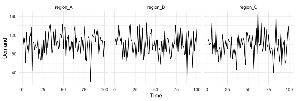
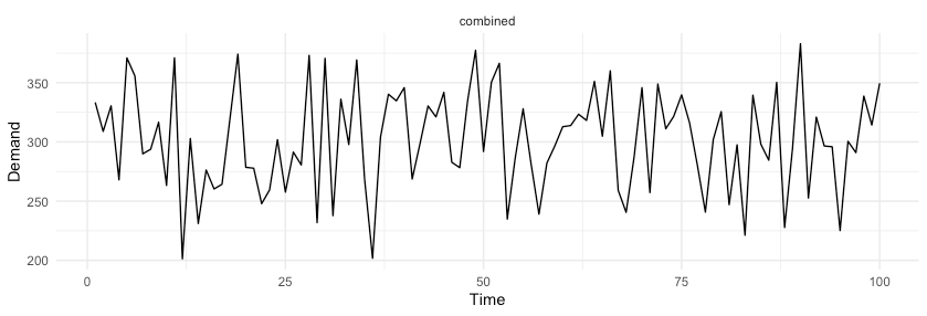
Although data aggregations can help with getting more accurate global forecasts, actions done on aggregated data can lead to inefficient mobilization. It is best to go for a solution where the unit of forecasting matches the unit of decision making.  

Choosing an optimizer

One benefit of using ML algorithms is that they provide more accurate expectations of what will happen given the input data. Nonetheless, ML algorithms are often simply a building block in a larger system that consumes predictions and attempts to generate a set of optimal actions. Mixed-integer programming (MIP) or reinforcement learning (RL)-based solutions are great in building systems that focus on reward maximization under specific business constraints. 

We decided to pursue a MIP approach given that it was easy to formalize, implement, and explain to stakeholders, and we have a lot of expertise in the domain. The optimizer has a custom objective function of minimizing undersupply with several constraints. The objective itself is very flexible and can be specified to favor either profitability or growth, depending on the business requirements. In the optimizer, we generally encoded a few global constraints:

• Never allocate more than one incentive in a particular region-time unit.
• Never exceed the maximum allowable budget set by our finance and operations partners.

Depending on requirements, we might also have different regional or country constraints, such as having different budgets, custom penalties, exclusion criteria for which units should not be included in the optimization, or incentive constraints that are guided by variability of the inputs. 

Dealing with uncertainty

Uncertainty in the inputs plays an important role in how the optimizer allocates incentives when resources are limited. To demonstrate, Figure 3, below, displays the distribution of the hypothesized supply and demand imbalance in two cities.

If the optimizer knows nothing about uncertainty, it ends up with two issues. First, it will lack understanding that supply and demand balance can go from a spectrum of extreme undersupply to extreme oversupply. If the optimizer is set up to optimize under some preset thresholds, it would miss the chance to optimize for City B because the mean of the distribution is above zero. 

The second issue is that it would end up over-allocating resources in places where our forecasts are uncertain. Our forecasts tend to be noisiest in the long tail of small regions that have few Dashers and few orders. Because the count of these regions is large and they exhibit high variance, if we don’t explicitly account for this uncertainty we are more likely to generate estimates that by chance will have high undersupply, and thus over-allocate incentives to places that exhibit high variance relative to places that have low variance. 

To address the issue of variance, we generate expected estimates of hours gap from forecasts using a resampling process. By performing resampling, we essentially measure the impact of undersupply in the context of the likelihood of that happening. For example, in Figure 3, above, City B has only a 34% chance of being undersupplied. However, if that happens, we can more accurately estimate the impact of sizable changes in undersupply. Either of these approaches lead to a more optimal decision in incentive allocation instead of simply using mean estimates from upstream forecasting inputs.  

Reliability and maintainability improvements

DoorDash has grown tremendously in the last year. More than 70% of the people at DoorDash joined in the 2020-21 period. This generally brought a wave of new engineering, product, platform, and infrastructure-related projects to help with continued growth, expansion, and scalability. For example, we had dozens of internal projects that related to breaking down our monolith and adopting a more microservice oriented architecture. We had hundreds of small and large projects related to product improvements or new vertical launches. Many of these projects came with changes in our data models and in our data generation and collection processes. Unfortunately, ML models can be terribly unreliable when the ecosystem for how data gets produced and exposed is constantly shifting, so we needed to make some changes to enhance the reliability of our system.

Decoupling data dependency chains

We could use many different data sources and encode hundreds of features to build a model that has high performance. Although that choice is very appealing and it does help with creating a model that performs better than one that has a simple data pipeline, in practice it creates a system that lacks reliability and generates a high surface area for feature drift, where the distribution of the inputs changes over time. Hence, when building our forecasting models, we went for simplicity and reliability first. This strategy also helped us move more quickly towards creating an end-to-end mobilization system.

	Complex pipeline	Simple pipeline
Performance relative to naive (in 1 month)	Great	Average
Performance relative to naive (in 2 months)	Average	Average
Performance relative to naive (in >3 months)	Terrible	Average
Remodeling Burden	High	Low
Oncall Burden	High	Low

To manage complexity and shifts in how data gets exposed, we did two things. First, we decoupled data pipelines from each other into separate business domains. Now, when someone is working on improving the signal for the inputs used in forecasting, they do not need to be overwhelmed by monolithic queries and data pipelines. Instead, a developer works on an isolated pipeline and only needs to ensure that aggregations are done on an appropriate entity. 

The second thing we did was to remove intermediary data dependencies. We recognized that if our input signals come from ETL jobs with very long dependency chains in their directed acyclic graphs (DAGs), we would increase our surface areas for failures. Hence, we would aspire to rely on primary tables thoroughly vetted by our Business Intelligence team or a copy of production data sources for which the data generation is not hidden behind complex ETLs. 

Focus on experimentation

One of the best ways to test if our system is maintainable is to simply check on the iteration speed with which we can push new changes and launch experiments without creating bugs or introducing regressions. At DoorDash, we perform many experiments to determine whether a feature is working as intended. This generally means that we put a lot more emphasis on measuring the software quality by how quickly we can extend and deliver on new functionality. Unsurprisingly, if experiments are challenging to launch and new features are difficult to test, we have failed in our goal. 

Similarly, if a system stays unchanged over a long period of time (e.g., six months or more), it would also be an indication that something is wrong, because it means we created a system that is rigid and does not invite improvements, ideation, and experimentation. Continuous experimentation is a forcing function towards adopting better practices, such as relying on a CI/CD system for automation, setting up library dependency management, decoupling the code into business domains, and adding testing, alerting, and documentation. 

Results

Implementing this mobilization system let us more accurately allocate incentives to regional-time units that benefited most from the improved supply and demand balance. The system resulted in a better experience for our customers, as our metrics showed reductions in delivery times, cancelations, and extreme lateness. For Dashers, we were able to ensure that incentives are allocated in places where they are needed most. For merchants, we drove the overall order cancellations down. Moreover, due to improvements in forecasting accuracy, we were also able to more reliably hit budget expectations and observed less variability in spending decisions. Because of reliability improvements, we were able to get to a point where our experimentation velocity on the incentive mobilization system rapidly increased.

Conclusion

Problems that deal with optimizing a system under constraints benefit immensely from aligning on metrics that estimate the impact of actions at an appropriate level of aggregation. If forecasts are done daily, but optimization actions are taken sub-daily, decision making will likely be suboptimal. 

Secondly, we generally recommend decoupling forecasting components from decision-making components. Most optimization systems work better if the inputs have stable statistical properties where the forecast predictions are unbiased estimates. For example, it can be tempting to start using an asymmetric loss function in forecasting to align with whether we care more about underpredicting or overpredicting the output. Although this approach is perfect for a variety of problems where the output of an ML model is immediately used to drive the decision, for problems where the ML predictions are simply another input into a broader optimization engine, it is best to generate unbiased predictions. Instead, it is better to let an optimization engine handle tradeoffs. 

If you are passionate about building ML applications that impact the lives of millions of merchants, Dashers, and customers in a positive way, consider joining our team.

Acknowledgements

Many thanks to Jared Bauman and Dan Madwed for helping brainstorm the architecture of the new system, Gary Ren for guiding us through the complexity of Supply-Demand engineering components, Henry Liao for streamlining experimentation, and Matthew Ferro and Eugene Braude for pushing for increased automation.