Addressing the Challenges of Sample Ratio Mismatch in A/B Testing

Experimentation isn’t just a cornerstone for innovation and sound decision-making; it’s often referred to as the gold standard for problem-solving, thanks in part to its roots in the scientific method. The term itself conjures a sense of rigor, validity, and trust. Yet as powerful as experimentation is, its integrity can be compromised by overlooked details and unforeseen challenges. One of these challenges is sample ratio mismatch, or SRM. 

SRM represents one of the most egregious data quality issues in A/B tests because it fundamentally compromises the basic assumption of random assignment. For example, if two reasonably sized groups are expected to be split 50/50, but instead show a 55/45 split, the assignment process likely is compromised. This means there is a strong possibility that any experimental results and decisions based on them will not be valid.

At DoorDash, we constantly innovate and experiment. To do so effectively, we had to find ways to reduce our SRM rate. In this post, we explore some of the common examples of SRM failures we experienced, the solutions we've implemented to solve these issues, and how we raised awareness of these solutions internally to dramatically reduce our SRM rate. 

Figure 1: If we have two groups that are expected to have a distribution of 50/50, we expect the SRM check would pass if that 50/50 split is indeed observed. We should be concerned, however, if there is instead a split of 55/45.

Cautionary tales of faux gains and real losses

Example 1: The $10 Million Mirage

Imagine that your target is to improve weekly revenue per user. After setting up the experiment with a 50/50 split between control and treatment groups, you run the experiment for a week and see that revenue has improved 2% — a $200,000 weekly incremental revenue impact. Annualized, this results in more than $10 million per year. High-fives are exchanged and your team is already setting its sights on the next big project.

Fortunately, a more observant experimenter has noticed that the SRM check failed. Instead of a 50/50 split between treatment and control, there actually was a 49.5/50.5 split — more than enough to trigger an SRM failure. Careful examination shows that the root cause for the failure is that all employees were exposed to the treatment. Almost every customer-focused company has an internal practice of dogfooding in which internal employees get the latest features by default. Because employees engage with the product much more frequently than outside users, the ~1% contribution to the total sample was enough to skew the metrics. The team’s jubilation over a $10 million win was tragically premature.

Segment	Experiment Group	Number of samples	7 day revenue value/user	Reported Incremental Impact
All Users	Control	500,000	$10	$0
All Users	Treatment	500,000	$10
Employees	Treatment	10000	$30	$200,000

Table 1: In this experiment, there is a  49.95/50.05 between control and treatment groups. The imbalance is accidental, driven purely by including employees in the treatment group. Because employees engage with the product more, they skew the revenue impact by 2%, leading to the reported weekly $200,000 impact. When the employee segment is excluded, the real incremental impact is $0.

Note that a small change in the absolute size of the groups (1%) can introduce a very large change in the experiment metric (2%), which means that the size of the SRM doesn’t set a ceiling on its impact on the metric readout. Although the example above is fictitious, we have observed that on our platform experiments that have SRM have twice as many statistically significant metrics. Simply put, by turning a blind eye to imbalance, teams could erroneously double their rate of “statistically significant” findings, leading to potentially faulty conclusions. 

Example 2: The bugfix bias

Bug fix handling is another area in which users can inadvertently introduce SRM. Imagine, for example, that there’s a bug in the implementation of a recently introduced new treatment. An engineer detects that bug and fixes it mid-experiment. They subsequently adjust the experiment’s start date so that it does not include metric data collected prior to the bug fix. 

Figure 2: SRM imbalance introduced after mid-experiment bug fix 

Figure 2 shows the time lapse of exposure allocation change. Because users don’t forget history, the introduced bug leads to an uneven distribution that deviates from the expected sample ratio; low-intent users likely have left the platform while remaining treatment users have decided to stay. This imbalance leads both to SRM and pre-experimental bias in how results from this experiment can be interpreted.

The solution to this problem is to reshuffle the exposure for both control and treatment after the bug gets fixed. Restarting the experiment through reshuffling resolves the imbalance and brings control and treatment groups back to the same starting point.

Figure 3: Reshuffling experiment after bug fix resolves SRM

These are just two examples of how SRM can slip into experimentation. Unfortunately,  there is general agreement across the industry that SRM is easy to detect, but it is excruciatingly hard to diagnose and correct, even for seasoned experimenters. SRM can be driven by data quality issues, experiment configuration problems, incorrect filtering when joining data, improper rollouts/rollback procedures, interaction between experiments, inconsistent definitions for ConsumerIds (UUID vs. incremental ids), and any number of additional issues. Our challenge has been to create solutions to help our experimenters avoid, identify, and correct SRM.

Solutions from the trenches

At DoorDash, we have pursued several approaches to reduce the platform’s rate of SRM, including innovating on methodology for how we diagnose SRM, improving our real-time observability and alerting, and focusing on education and awareness. 

Statistical approaches for identifying imbalance

The most common approach for identifying SRM is to use a chi-square test that can quickly detect when something is wrong. These tests, however, can’t help identify why an imbalance has happened. So, as a follow up, some platforms allow experimenters to perform “eyeball statistics.” This allows segmenting data to understand which attribute might be driving the imbalance. For example, information collected and randomized upon platform usage could be segmented into Android and iOS to allow a visual check for irregularities. 

An improvement on such ad-hoc segmentation would be to run a chi-square test repeatedly on segment subpopulations or to run permutation tests against contingency tables. The latter  approach bests a chi-square test because it can flag which user segments are driving the imbalance and provides inferential statistics for use in making decisions. That said, there are three problems with running permutation tests tests or ad hoc chi-square tests:

• They don’t generate orthogonal effects. Figure 3 below shows an example in which country and platform segments are analyzed separately, leading to imbalances in both. For example, the imbalance might be caused by Android exposures, yet because the U.S. has more Android users than other parts of the world, the country attribute will also be flagged as an imbalance. Lack of orthogonal effects is the biggest disadvantage of current methods. 
• They don’t provide a good tradeoff between false positives and the power to detect SRM. Running permutation tests and chi-square tests against dozens of segments requires aggressive p-value corrections, thus reducing the sensitivity of the SRM check.
• They are computationally inefficient. Running permutation testing at scale with tens of thousands of daily checks can quickly generate a very inefficient infrastructure footprint. 

Instead, we wanted an approach that allows us to generate orthogonal effects, scales well, and doesn’t sacrifice power.

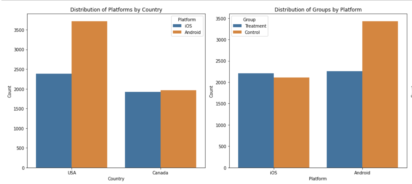
Figure 4: To demonstrate why orthogonal effects are important, note that Android is the root issue leading to imbalance. But because the U.S. has more Android users than other countries, an experimenter might mistakenly assume that the problem can be attributed to the user country. 

Our approach: Regression is all we need

When we randomly assign users to treatment and control groups, we assume that there is nothing else in the world but randomness driving those assignments. As illustrated in Figure 5 below, if we were to assign an estimator to check for any relationships between user attributes before randomization and assignment, there should be zero correlation or regression coefficients. 

Figure 5: Attributes collected prior to randomization should have no impact on treatment assignment. 

One estimator that provides us with orthogonalization properties and generates simple to interpret statistics that allow us to verify if something is related to treatment assignment is linear regression. 

We will use two dimensions to more clearly explain how to use linear regression to identify imbalance. Let’s assume that we have two attributes we collect at the time of randomization: 

• Country: USA, Canada, Australia
• Platform: Web, iOS, Android

We will test our approach with three scenarios:

• No imbalance
• Imbalance due to country=Australia
• Imbalance due to country=Australia OR platform=Web

Figure 6: In scenario 1, there is no imbalance. In Scenario 2, there is  an imbalance driven by having a split of 80/20 instead of 50/50 in Australia. In Scenario 3, there is  an imbalance driven by both the Australia segment and the Android segment, which also has an 80/20 split.

import pandas as pd
import numpy as np
import statsmodels.formula.api as smf
def generate_data(n,
                  platforms=["iOS", "Android", "Web"],
                  countries=["USA", "AUS", "CAN"]):
    np.random.seed(42)
    expected_distribution = [0.5, 0.5]
    experiment_groups = [1, 0]
    df = pd.DataFrame(
        {
            "user_id": range(1, n + 1),
            "platform": np.random.choice(platforms, size=n),
            "country": np.random.choice(countries, size=n),
        }
    )
    # Scenario 1: No imbalance
    df["scenario_1"] = np.random.choice(experiment_groups, size=n, p=expected_distribution)
    # Scenario 2: Australia 80/20 imbalance
    df["scenario_2"] = df["scenario_1"]
    mask_2 = df["country"] == "AUS"
    df.loc[mask_2, "scenario_2"] = np.random.choice(experiment_groups, size=sum(mask_2), p=[0.8, 0.2])
    # Scenario 3: Australia or Android 80/20 imbalance
    df["scenario_3"] = df["scenario_1"]
    mask_3 = (df["country"] == "AUS") | (df["platform"] == "Android")
    df.loc[mask_3, "scenario_3"] = np.random.choice(experiment_groups, size=sum(mask_3), p=[0.8, 0.2])    
    return df

In this code snippet, we generate data with three randomization options: one with completely random assignment, one where the distribution skew is driven by platform, and one where the distribution skew is driven by country or platform. 

Fundamentally, if we want to understand what attributes are related to treatment assignment, we simply have to fit a regression with the following form:

is_treatment ~ country + platform

The code below allows us to run this regression.

def run_model(df, scenario_name):
    # center the outcome variable around expected ratio
    df['is_treatment'] = df[scenario_name] - 0.5
    formula = "is_treatment ~ 1 + platform + country"
    # fit the regression 
    m = smf.glm(formula, data=df).fit(cov_type="HC1")
    # get the p-values for the main effect using a Wald test
    wald_p_values = m.wald_test_terms(scalar=True).table
    return wald_p_values

Here we run a regression to explain if treatment assignment is a function of platform and country variables. Given that we’re interested only in the main effects of those variables, we follow it up with a Wald test that asks: Is the main effect of a particular predictor related to treatment assignment?

Note that when we run the regression, we are interested in main effects (e.g., “Is there a main effect of the platform on treatment assignment?”), so we use a Wald test to get the p-values for the main effect. Figure 7 shows the Wald test output for each of the three scenarios. We can immediately draw these conclusions:

• In Scenario 1, none of the attributes are related to treatment assignment.
• In Scenario 2, we can see that country has a very low p-value. There is a main effect from country, but we don’t know yet which specific country segment is responsible for the imbalance.
• In Scenario 3, we can see that both platform and country are drivers of imbalance. 

Figure 7: The Wald test results show: In scenario 1, none of the attributes are related to treatment assignment. In scenario 2, only country is related to treatment assignment (p<0.0001) and in scenario 3 both platform and country are predictive of treatment assignment (p<0.0001). 

Note that our internal implementation is more complex. The example process described so far only allows us to find the main effects. Internally, we apply a recursive algorithm to eliminate subsets of the data that contribute most to imbalance, similar to what an experimenter would do in the process of salvaging data from SRM. Moreover, we apply a correction to p-values when we perform multiple checks and handle a variety of edge cases, such as when a segment has zero variance or the regression is not invertible because of perfect multicollinearity. 

Optimizations

As shown in the code snippet below, an important optimization we can do relies on weighted regression when performing the computation. Using weights in regression allows efficient scaling of the algorithm, even when interacting with large datasets. With this approach, we don’t just perform the regression computation more efficiently, we also minimize any network transfer costs and latencies and can perform much of the aggregation to get the inputs on the data warehouse. 

df_aggregated = df.groupby(['country', 'platform', 'scenario_1'], as_index=False).size()
model1 = smf.glm(formula, data=df, freq_weights=df.size.df_aggregated).fit(cov_type="HC1")

In this example, we aggregate the data to the platform, country, and experiment group level. This aggregation allows us to reduce the data size from millions to hundreds of rows, making the SRM computation many orders of magnitude more efficient. This aggregation is done on the data warehouse side.

Extensions

After ruling out all causes of imbalance, an extension of this methodology would be to use the regression approach to correct for SRM, thus salvaging the collected data. This should be done only after clear causes of imbalance have been identified. To apply correction, you simply need to fit a regression with this form:

metric_outcome  ~ is_treatment + country + platform 

Adding the two regressor variables not only corrects results for SRM, but could also contribute to variance reduction because the additional covariates could explain some of the variance in the metric outcome. 

Observability

DoorDash also has explored ways to give users better observability on experiment exposures beyond the statistical methods mentioned previously. Experiment exposures are one of our highest volume events. On a typical day, our platform produces between 80 billion and 110 billion exposure events. We stream these events to Kafka and then store them in Snowflake. Users can query this data to troubleshoot their experiments. However, there are some issues with the current tools:

1. There is a lag on the order of tens of minutes between when the exposures are created and when they are available for querying in Snowflake.
2. The queries take a long time to run on Snowflake, even after we apply partitioning. Running complex queries takes even longer.

We want to give users an easy-to-consume dashboard to let them monitor and observe experiment exposures in real time. This allows users to gain immediate insights into the performance and health of their ongoing experiments. As an added benefit, the dashboard reduces our reliance on Snowflake to troubleshoot experiments thereby reducing overall operational costs.

We needed to do two things to create the dashboards. First, we had to aggregate the exposure stream across different dimensions. We included dimensions like experiment name, experiment version, variant, and segment, which represents the population group for the sample as defined when setting up the experiment. For this task, we used Apache Flink, which supports stream processing and provides event-time processing semantics. Supported internally at DoorDash, Flink is used by many teams to run their processing jobs on streaming data. We use Flink’s built-in time-window-based aggregation functions on exposure time. We then send this aggregated data to another Kafka topic. 

Next, we had to save the data that is aggregated by the time-window into a datastore. We wanted an analytics OLAP datastore with low latency. For this we used Apache Pinot. Pinot is a real-time distributed OLAP datastore which can ingest data from streaming sources like Kafka, scale horizontally, and provide real-time analytics with low latency. We rely on Pinot’s built-in aggregation functions to produce the final results, which are fed into the user dashboards to provide various visualizations. Figure 8 below shows the high-level overview of our solution:

Figure 8: Here we summarize our real-time stream processing.

We added another layer of transparency by embedding these dashboards into our experiment configuration platform. With this tool, users can quickly troubleshoot a number of issues associated with SRM, including:

• Did I launch one treatment variant sooner than another?
• Are there more exposures in one group versus another?
• Are there any anomalies present in the time series of exposure logs?

Below are sample charts from our dashboards.

Figure 9: This shows the timeline of exposure count by variant. A user can access this data within minutes after launching an experiment.

Figure 10: Visualizations of the distribution of exposures by each variant allow a user to check for any major irregularities. 

Real-time insights not only help in diagnosing issues with experiments but also generate greater confidence that a rollout is proceeding as expected.

Alerting

To further minimize the rate of SRM occurrences, users can subscribe to an experiment health check alert system that notifies them quickly — often within 24 hours — if an imbalance is detected within their experiment. This allows for timely, proactive adjustments that can virtually eliminate the need to discard otherwise valuable data down the line due to invalidated results.

Figure 11: When setting up an experiment, users can subscribe to our alert system. 

Education is key: The role of awareness in reducing SRM

In our quest to reduce the incidence of SRM on the platform, we’ve explored and implemented a variety of technical solutions — from real-time monitoring systems to new algorithms that identify imbalance sources. While these advancements have been crucial in minimizing SRM, we found that human intervention through awareness and education remains indispensable and moves the needle most. Recognizing this gap, we initiated a multi-pronged educational approach, including:

• Training sessions: We organized an internal bootcamp focused on best practices for experiment configuration, highlighting how to prevent imbalance due to simple configuration problems.
• Documentation: We provided comprehensive guides with case studies that a non-technical person can understand. We even renamed the terminology internally from “Sample Ratio Mismatch,” which is a technical mouthful, to “Imbalance Check.”
• Stronger language: We changed documentation language and how we communicate SRM failures to be more in line with the size of impact that it has on decision making. Although there are rare cases in which SRM failures can be overlooked, the revised language emphasizes that imbalanced experiment results can’t be trusted. 
• Proactive user engagement: The reactive nature of problem-solving poses a challenge to minimizing SRM. Users may only become aware of SRM after they encounter the problem, which often leads to delayed actions. Instead of waiting for users to join our training session or open the documentation and diagnostic tools, we engage them early through team-specific knowledge share sessions.

Sometimes the best solutions aren't just about building a better mousetrap, but instead ensuring that everyone knows how to use the new tools effectively. For us, education and awareness have made all the difference. Writing this blogpost is itself an attempt to push for greater awareness and education.    

Results

Within six months of starting our work, we saw a 70% drop in SRM incidents on the platform. This means that hundreds of experiments which might have been plagued by incorrect conclusions instead lead to legitimate results. Beyond the numbers, there has been a palpable shift in team dynamics. With heightened awareness, A/B tests are set and reviewed more thoroughly and executed more successfully. Teams no longer must expend valuable resources and experimental capacity on restarting tests or reconciling unexpected outcomes caused by imbalance failures.

Future Work

Although we have made great progress toward reducing the incidence of SRM at DoorDash, we believe even more improvements can be made through real-time observability, automatic correction, and standardization.

• Real-time observability can be improved by integrating more tightly with the algorithms used in diagnostic checking. It is computationally inexpensive to run Wald tests and weighted regression on count data, so we would like to run it on the query outputs from Pinot whenever a user examines real time exposures.
• Automatic correction will allow us to fix common SRM problems and adjust experiment results without compelling the user to take any additional action. As shown previously, if we can identify the source of imbalance, we can often salvage the analysis result by adding additional covariates to our estimator.
• Standardization offers a safeguard against common pitfalls, thereby reducing the likelihood of user errors. For example, if a user fixes a bug and relaunches an experiment, our system could proactively identify potential repercussions of the changes and adjust the strength of warnings or guidelines accordingly.

Through such measures, we can further elevate the robustness and credibility of experimental results.

Acknowledgements

Many thanks to Drew Trager, Sharon Weng, Hassan Djirdeh, Yixin Tang, Dave Press, Bhawana Goel, Caixia Huang, Kevin Tang, and Qiyun Pan, who have been instrumental in their feedback, execution, and collaboration across many of the initiatives outlined above. Finally, many thanks to the Eng Enablement team: Janet Rae-Dupree, Robby Kalland, and Marisa Kwan for their continuous support in reviewing and editing this article. 

If you’re passionate about building innovative products that make positive impacts in the lives of millions of merchants, Dashers, and customers, consider joining our team.