Cassandra Unleashed: How We Enhanced Cassandra Fleet’s Efficiency and Performance

In the realm of distributed databases, Apache Cassandra stands out as a significant player. It offers a blend of robust scalability and high availability without compromising on performance. However, Cassandra also is notorious for being hard to tune for performance and for the pitfalls that can arise during that process. The system's expansive flexibility, while a key strength, also means that effectively harnessing its full capabilities often involves navigating a complex maze of configurations and performance trade-offs. If not carefully managed, this complexity can sometimes lead to unexpected behaviors or suboptimal performance.

In this blog post, we walk through DoorDash’s Cassandra optimization journey. I will share what we learned as we made our fleet much more performant and cost-effective. Through analyzing our use cases, we hope to share universal lessons that you might find useful. Before we dive into those details, let’s briefly talk about the basics of Cassandra and its pros and cons as a distributed NoSQL database. 

What is Apache Cassandra?

Apache Cassandra is an open-source, distributed NoSQL database management system designed to handle large amounts of data across a wide range of commodity servers. It provides high availability with no single point of failure. Heavily inspired by Amazon’s 2007 DynamoDB, Facebook developed Cassandra to power its inbox search feature and later open-sourced it. Since then, it has become one of the preferred distributed key-value stores. 

Cassandra pros

• Scalability: One of Cassandra’s most compelling features is its exceptional scalability. It excels in both horizontal and vertical scaling, allowing it to manage large volumes of data effortlessly.
• Fault tolerance: Cassandra offers excellent fault tolerance through its distributed architecture. Data is replicated across multiple nodes, ensuring no single point of failure.
• High availability: With its replication strategy and decentralized nature, Cassandra guarantees high availability, making it a reliable choice for critical applications.
• Flexibility: Cassandra supports a flexible schema design, which is a boon for applications with evolving data structures.
• Write efficiency: Cassandra is optimized for high write throughput, handling large volumes of writes without a hitch.

Cassandra cons

• Read performance: While Cassandra excels in write efficiency, its read performance can be less impressive, especially in scenarios involving large data sets with frequent reads at high consistency constraints.
• Expensive to modify data: Because Cassandra is a log structured merge tree where the data written is immutable, deletion and updates are expensive. Especially for deletes, it can generate tombstones that impact performance. If your workload is delete- and update-heavy, a Cassandra-only architecture might not be the best choice.
• Complexity in tuning: Tuning Cassandra for optimal performance requires a deep understanding of its internal mechanisms, which can be complex and time-consuming.
• Consistency trade-off: In accordance with the CAP theorem, Cassandra often trades off consistency for availability and partition tolerance, which might not suit all use cases.

Cassandra’s nuances

The nuances surrounding Cassandra's application become evident when weighing its benefits against specific use case requirements. While its scalability and reliability are unparalleled for write-intensive applications, one must consider the nature of their project’s data and access patterns. For example, if your application requires complex query capabilities, systems like MongoDB might be more suitable. Alternatively, if strong consistency is a critical requirement, CockroachDB could be a better fit.

In our journey at DoorDash, we navigated these gray areas by carefully evaluating our needs and aligning them with Cassandra's capabilities. We recognized that, while no system is a one-size-fits-all solution, with meticulous tuning and understanding Cassandra's potential could be maximized to meet and even exceed our expectations. The following sections delve into how we approached tuning Cassandra — mitigating its cons while leveraging its pros — to tailor it effectively for our data-intensive use cases.

Dare to improve

Because of DoorDash’s fast growth, our usage of Cassandra has expanded rapidly. Despite enhancing our development speed, this swift growth left a trail of missed opportunities to fine-tune Cassandra’s performance. In an attempt to seize some of those opportunities, the Infrastructure Storage team worked closely with product teams on a months-long tuning effort. The project has delivered some amazing results, including: 

• ~35% in cost reduction for the entire Cassandra fleet 
• For each $1 we spend, we are able to process 59 KB of data per second vs. 23 KB, a whopping 154% unit economics improvement

In the following section, we will explore specific examples from our fleet that may be applicable to other use cases. 

Design your schema wisely from the beginning

The foundational step to ensuring an optimized Cassandra cluster is to have a well-designed schema. The design choices made at the schema level have far-reaching implications for performance, scalability, and maintainability. A poorly designed schema in Cassandra can lead to issues such as inefficient queries, hotspots in the data distribution, and difficulties in scaling. Here are some key considerations for designing an effective Cassandra schema:

• Understand data access patterns: Before designing your schema, it’s crucial to have a clear understanding of your application's data access patterns. Cassandra is optimized for fast writes and efficient reads, but only if the data model aligns with how the data will be accessed. Design your tables around your queries, not the other way around.
• Effective use of primary keys: The primary key in Cassandra is composed of partition keys and clustering columns. The partition key determines the distribution of data across the cluster, so it’s essential to choose a partition key that ensures even data distribution while supporting your primary access patterns. Clustering columns determine the sort order within a partition and can be used to support efficient range queries.
• Avoid large partitions: Extremely large partitions can be detrimental to Cassandra's performance. They can lead to issues like long garbage collection pauses, increased read latencies, and challenges in compaction. Design your schema to avoid hotspots and ensure a more uniform distribution of data.
• Normalization vs. denormalization: Unlike traditional relational database management systems, or RDBMS, Cassandra does not excel at joining tables. As a result, denormalization is often necessary. However, it’s a balance; while denormalization can simplify queries and improve performance, it can also lead to data redundancy and larger storage requirements. Consider your use case carefully when deciding how much to denormalize.
• Consider the implications of secondary indexes: Secondary indexes in Cassandra can be useful but come with trade-offs. They can add overhead and may not always be efficient, especially if the indexed columns have high cardinality or if the query patterns do not leverage the strengths of secondary indexes.
• TTL and tombstones management: Time-to-live, or TTL, is a powerful feature in Cassandra for managing data expiration. However, it’s important to understand how TTL and the resulting tombstones affect performance. Improper handling of tombstones can lead to performance degradation over time. If possible, avoid deletes.
• Update strategies: Understand how updates work in Cassandra. Because updates are essentially write operations, they can lead to the creation of multiple versions of a row that need to be resolved at read time, which impacts performance. Design your update patterns to minimize such impacts. If possible, avoid updates.

Choose your consistency level wisely

Cassandra's ability to configure consistency levels for read and write operations offers a powerful tool to balance between data accuracy and performance. However, as with any powerful feature, it comes with a caveat: Responsibility. The chosen consistency level can significantly impact the performance, availability, and fault tolerance of your Cassandra cluster, including the following areas:

• Understanding consistency levels: In Cassandra, consistency levels range from ONE (where the operation requires confirmation from a single node) to ALL (where the operation needs acknowledgment from all replicas in the cluster). There are also levels like QUORUM (requiring a majority of the nodes) and LOCAL_QUORUM (a majority within the local data center). Each of these levels has its own implications on performance and data accuracy. You can learn more about those levels in the configurations here. 
• Performance vs. accuracy trade-off: Lower consistency levels like ONE can offer higher performance because they require fewer nodes to respond. However, they also carry a higher risk of data inconsistency. Higher levels like ALL ensure strong consistency but can significantly impact performance and availability, especially in a multi-datacenter setup.
• Impact on availability and fault tolerance: Higher consistency levels can also impact the availability of your application. For example, if you use a consistency level of ALL, and even one replica is down, the operation will fail. Therefore, it's important to balance the need for consistency with the potential for node failures and network issues.
• Dynamic adjustment based on use case: One strategy is to dynamically adjust consistency levels based on the criticality of the operation or the current state of the cluster. This approach requires a more sophisticated application logic but can optimize both performance and data accuracy.

Tune your compaction strategy (and bloom filter)

Compaction is a maintenance process in Cassandra that merges multiple SSTables, or  sorted string tables, into a single one. Compaction is performed to reclaim space, improve read performance, clean up tombstones, and optimize disk I/O.

Users should choose from three main strategies to trigger compaction in Cassandra users based on their use cases. Each strategy is optimized for different things: 

1. Size-tiered compaction strategy, or STCS
   • Trigger mechanism:
     • The strategy monitors the size of SSTables. When a certain number reach roughly the same size, the compaction process is triggered for those SSTables. For example, if the system has a threshold set for four, when four SSTables reach a similar size they will be merged into one during the compaction process.
   • When to use:
     • Write-intensive workloads
     • Consistent SSTable sizes
   • Pros:
     • Reduced write amplification
     • Good writing performance
   • Cons:
     • Potential drop in read performance because of increased SSTable scans
     • Merges older and newer data over time
     • You must leave much larger spare disk to effectively run this compaction strategy
2. Leveled compaction strategy, or LCS
   • Trigger mechanism:
     • Data is organized into levels. Level 0 (L0) is special and contains newly flushed or compacted SSTables. When the number of SSTables in L0 surpasses a specific threshold (for example 10 SSTables), these SSTables are compacted with the SSTables in Level 1 (L1). When L1 grows beyond its size limit, it gets compacted with L2, and so on.
   • When to use:
     • Read-intensive workloads
     • Needing consistent read performance
     • Disk space management is vital
   • Pros:
     • Predictable read performance because of fewer SSTables
     • Efficient disk space utilization
   • Cons:
     • Increased write amplification
3. TimeWindow compaction strategy, or TWCS
   • Trigger mechanism:
     • SSTables are grouped based on the data's timestamp, creating distinct time windows such as daily or hourly. When a time window expires — meaning we've moved to the next window — the SSTables within that expired window become candidates for compaction. Only SSTables within the same window are compacted together, ensuring temporal data locality.
   • When to use:
     • Time-series data or predictable lifecycle data
     • TTL-based expirations
   • Pros:
     • Efficient time-series data handling
     • Reduced read amplification for time-stamped queries
     • Immutable older SSTables
   • Cons:
     • Not suitable for non-temporal workloads
     • Potential space issues if data within a time window is vast and varies significantly between windows

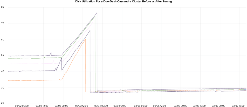
In our experience, unless you are strictly storing time series data with predefined TTL, LCS should be your default choice. Even when your application is write-intensive, the extra disk space required by progressively large SSTables under STCS makes this strategy unappealing. LCS is a no-brainer in read-intensive use cases. Figure 2 below shows the amount of disk usage drop after switching compaction strategy and cleanups.

It’s easy to forget that each compaction strategy should have a different bloom filter cache size. When you switch between compaction strategies, do not forget to adjust this  cache size accordingly. 

• STCS default bloom filter setting: The default setting for STCS usually aims for a balance between memory usage and read performance. Because STCS can lead to larger SSTables, the bloom filter might be configured as slightly larger than what would be used in LCS to reduce the chance of unnecessary disk reads. However, the exact size will depend on the Cassandra configuration and the specific workload.
• LCS default bloom filter setting: LCS bloom filters generally are smaller because SSTables are managed in levels and each level contains non-overlapping data. This organization reduces the need for larger bloom filters, as it's less likely to perform unnecessary disk reads
• TWCS default bloom filter setting: Used primarily for time-series data, TWCS typically involves shorter-lived SSTables because of  the nature of time-based data expiry. The default bloom filter size for TWCS might be adjusted to reflect the data’s temporal nature of the data; it’s potentially smaller because of the predictable aging-out of SSTables.

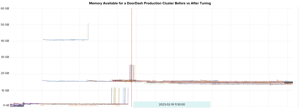
As a specific example, we switched one of our Cassandra clusters running on 3.11 from STCS to LCS as shown in Figure 3 below. However, we did not increase the bloom filter cache size accordingly. As a result, the nodes in that cluster were constantly running out of memory, or OOM due to the increased false positives rate for reads. After increasing bloom_filter_fp_chance from 0.01 to 0.1, plenty more OS Memory is spared, eliminating the OOM problem. 

To batch or not to batch? It’s a hard question

In traditional relational databases, batching operations is a common technique to improve performance because it can reduce network round trips and streamline transaction management. However, when working with a distributed database like Cassandra, the batching approach, whether for reads or writes, requires careful consideration because of its unique architecture and data distribution methods.

Batched writes: The trade-offs

Cassandra, optimized for high write throughput, handles individual write operations efficiently across its distributed nodes. But batched writes, rather than improving performance, can introduce several challenges, such as:

• Increased load on coordinator nodes: Large batches can create bottlenecks at the coordinator node, which is responsible for managing the distribution of these write operations.
• Write amplification: Batching can lead to more data being written to disk than necessary, straining the I/O subsystem.
• Potential for latency and failures: Large batch operations might exceed timeout thresholds, leading to partial writes or the need for retries.

Given these factors, we often find smaller, frequent batches or individual writes more effective, ensuring a more balanced load distribution and consistent performance.

Batched reads: A different perspective

Batched reads in Cassandra, or multi-get operations, involve fetching data from multiple rows or partitions. While seemingly efficient, this approach comes with its own set of complications:

• Coordinator and network overhead: The coordinator node must query across multiple nodes, potentially increasing response times.
• Impact on large partitions: Large batched reads can lead to performance issues, especially from big partitions.
• Data locality and distribution: Batching can disrupt data locality, a key factor in Cassandra's performance, leading to slower operations.
• Risk of hotspots: Unevenly distributed batched reads can create hotspots, affecting load balancing across the cluster.

To mitigate these issues, it can be more beneficial to work with targeted read operations that align with Cassandra’s strengths in handling distributed data.

In our journey at DoorDash, we've learned that batching in Cassandra does not follow the conventional wisdom of traditional RDBMS systems. Whether it's for reads or writes, each batched operation must be carefully evaluated in the context of Cassandra’s distributed nature and data handling characteristics. By doing so, we've managed to optimize our Cassandra use, achieving a balance between performance, reliability, and resource efficiency.

DataCenter is not for query isolation

Cassandra utilizes data centers, or DCs, to support multi-region availability, a feature that's critical for ensuring high availability and disaster recovery. However, there's a common misconception regarding the use of DCs in Cassandra, especially among those transitioning from traditional RDBMS systems. It may seem intuitive to treat a DC as a read replica, similar to how read replicas are used in RDBMS for load balancing and query offloading. But in Cassandra, this approach needs careful consideration.

Each DC in Cassandra can participate in the replication of data; this replication is vital for the overall resilience of the system. While it's possible to designate a DC for read-heavy workloads — as we have done at DoorDash with our read-only DC — this decision isn't without trade-offs.

One critical aspect to understand is the concept of back pressure. In our setup, the read-only DC is only used for read operations. However, this doesn't completely isolate the main DC from the load. When the read-only DC experiences high load or other issues, it can create back pressure that impacts the main DC. This is because in a Cassandra cluster all DCs are interconnected and participate in the overall cluster health and data replication process.

For instance, if the read-only DC is overwhelmed by heavy or bad queries, it can slow down, leading to increased latencies. These delays can ripple back to the main DC, as it waits for acknowledgments or tries to manage the replication consistency across DCs. Such scenarios can lead to a reduced throughput and increased latency cluster-wide, not just within the read-only DC.

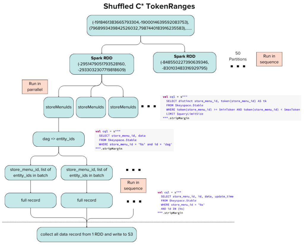
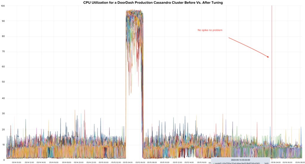
In one of our Cassandra clusters, we used its read-only DC to house expensive analytics queries that effectively take a daily snapshot of the tables. Because we treated the RO DC as complicated and isolated, as the number of tables grew the queries got more and more expensive. Eventually, the analytics job caused the RO DC to become pegged at 100% every night. This also started to impact the main DC. Working with the product team, we drastically optimized those batch jobs and created a better way to take the snapshot. Without going into too much detail, we utilized toke range to randomly walk the ring and distribute the load across the clusters.  Figure 4 below shows the rough architecture. 

The end result was amazing. The CPU spike was eliminated, enabling us to decommission the RO DC altogether. The main DC performance also noticeably benefited from this. 

GC tuning: Sometimes worth it

Within Cassandra, GC tuning, or garbage collection tuning, is a challenging task. It demands a deep understanding of garbage collection mechanisms within the Java Virtual Machine, or JVM, as well as how Cassandra interacts with these systems. Despite its complexity, fine-tuning the garbage collection process can yield significant performance improvements, particularly in high-throughput environments like ours at DoorDash. Here are some common considerations:

• Prefer more frequent young generation collections: In JVM garbage collection, objects are first allocated in the young generation, which is typically smaller and collected more frequently. Tuning Cassandra to favor more frequent young gen collections can help to quickly clear short-lived objects, reducing the overall memory footprint. This approach often involves adjusting the size of the young generation and the frequency of collections to strike a balance between reclaiming memory promptly and not overwhelming the system with too many GC pauses.
• Avoid old generation collections: Objects that survive multiple young gen collections are promoted to the old generation, which is collected less frequently. Collections in the old generation are more resource-intensive and can lead to longer pause times. In a database like Cassandra, where consistent performance is key, it's crucial to minimize old gen collections. This can involve not only tuning the young/old generation sizes but also optimizing Cassandra's memory usage and data structures to reduce the amount of garbage produced.
• Tune the garbage collector algorithm: Different garbage collectors have different characteristics and are suited to different types of workloads. For example, the G1 garbage collector is often a good choice for Cassandra, as it can efficiently manage large heaps with minimal pause times. However, the choice and tuning of the garbage collector should be based on specific workload patterns and the behavior observed in your environment.
• Monitor and adjust based on metrics: Effective GC tuning requires continuous monitoring and adjustments. Key metrics to monitor include pause times, frequency of collections, and the rate of object allocation and promotion. Tools like JMX, JVM monitoring tools, and Cassandra's own metrics can provide valuable insights into how GC is behaving and how it impacts overall performance.
• Understand the impact on throughput and latency: Any GC tuning should consider its impact on both throughput and latency. While more aggressive GC can reduce memory footprint, it might also introduce more frequent pauses, affecting latency. The goal is to find a configuration that offers an optimal balance for your specific workload.

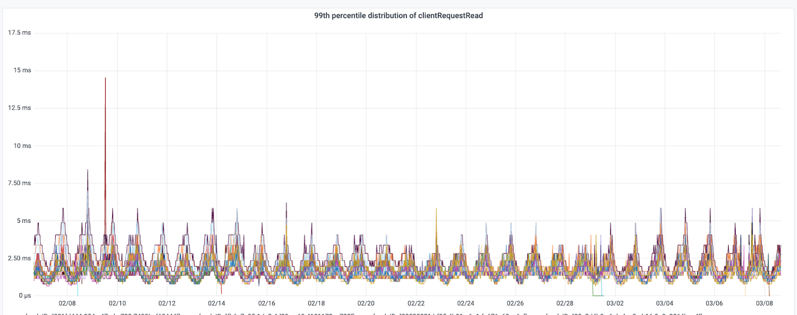
In our experience at DoorDash, we've found that targeted GC tuning, while complex, can be highly beneficial. By carefully analyzing our workloads and iteratively tuning our GC settings, we've managed to reduce pause times and increase overall system throughput and reliability. However, it's worth noting that GC tuning is not a one-time task but an ongoing process of observation, adjustment, and optimization. Figure 6 below shows provides an example of when we tuned our GC to achieve better P99 performance. 

Future work and applications

As we look toward the future at DoorDash, our journey with Apache Cassandra is set to deepen and evolve. One of our ongoing quests is to refine query optimizations. We're diving into the nuances of batch sizes and steering clear of anti-patterns that hinder efficiency.

Another challenge remaining is performance of the change data capture, or CDC. Our current setup with Debezium, paired with Cassandra 3, suffers from limitations in latency, reliability, and scalability. We're eyeing a transition to Cassandra 4 and raw clients, which offer better CDC capabilities. This shift isn't just a technical upgrade; it's a strategic move to unlock new realms of real-time data processing and integration.

Observability in Cassandra is another frontier we're eager to conquer. The current landscape makes it difficult to discern the intricacies of query performance. To bring these hidden aspects into the light, we're embarking on an initiative to integrate our own proxy layer. This addition, while introducing an extra hop in our data flow, promises a wealth of insights into query dynamics. It's a calculated trade-off, one that we believe will enrich our understanding and control over our data operations.

Acknowledgements 

This initiative wouldn’t be a success without the help of our partners, the DRIs of the various clusters that were tuned, including:

• Ads Team: Chao Chu, Deepak Shivaram, Michael Kniffen, Erik Zhang, and Taige Zhang
• Order Team: Cesare Celozzi, Maggie Fang, and Abhishek Sharma
• Audience Team: Edwin Zhang
• Menu & Data Team: Yibing Shi, Jonathan Brito, Xilu Wang, and Santosh Vanga

Thanks also to Levon Stepanian for helping track cost savings across AWS Infra and Instaclustr management fees. Finally, thank you for the support from the broader storage team and our Instaclustr partners.